Copper wire heating - ‘Hello World!’ example¶

Hello copper wire!

Physical formulation¶

Let us consider a thermally insulated cooper wire \(\Omega\) of length \(L\) and radius \(R\) with a straight centerline whose direction coincides with the \(+x\)-axis. The wire is subject to a voltage drop \(U\) connecting a heat pump control unit, which is located in a house cellar with the temperature \(T_\mathrm{c}\), with an external heat exchanger located outside at the ambient air temperature \(T_\mathrm{h}\). Our goal is to compute the equilibrium temperature distribution of the wire for the given parameters.

[168]:

%%tikz -l patterns -s 600,320
\input{fig/formulation.tikz};

../_images/HeatEquation1D_wire1d_4_0.png

FEniCS Implementation¶

Having clarified the basic formulation of the problem, we can start implementing it in FEniCS. First of all, we must import the fenics library into the python interface. Moreover, we import the pyplot library that is used for graph rendering. Finally, we will also need some features of the numpy package.

[169]:

# Import relevant modules:
import fenics as fe # 'import dolfin' does the same
import matplotlib.pyplot as plt
import numpy as np

Problem parameters¶

As a first step in the actual implementation, we need to specify electrical resistivity and heat conductivity of copper, our material of choice. Following table shows also some other materials for comparison. All the values are for the temperature around 20 °C and atmospheric pressure.

Material	Electrical resistivity \(\rho\ [\Omega \cdot \mathrm{m}]\)	Thermal conductivity \(k\ [\mathrm{W} \cdot \mathrm{m}^{-1} \cdot \math rm{K}^{-1}]\)
Copper	\(1.68\times10^{−8}\)	\(384.1\)
Silver	\(1.59\times10^{−8}\)	\(429\)
Stainless Steel	\(69.0\times10^{−8}\)	\(16\)–\(20\)
Glass	\(10^{11}\)–\(10^{15}\)	\(0.8\)–\(1.9\)

It is recommended to gather all the problem parameters at the beginning of the solution script file, let us follow it by specifying the geometeric, the environment, and the material parameters.

[170]:

# --------------------
# Parameters
# --------------------
# Geometric parameters:
L = 5.0  # Length of the wire [m]
R = 0.005 # Radius of the wire [m]
A = np.pi*R**2 # Cross-section area [m^2]

# Environment parameters:
T_c = 283 # Ambient temperature of the cellar [K]
T_h = 298 # Ambient temperature of the outside air [K]
U = 230 # Voltage drop [V]

# Material parameters:
rho = 1.68e-8 # Electrical resistivity of copper [Ω m]
k = 384.1 # Thermal conductivity of copper [W m^-1 K^-1]

Geometry of the problem¶

Next, we define the discretized geometry of our problem. There is always a possibility to use an external mesh defined in an .xml file. In our case, we use the predefined interval mesh provided directly by FEniCS environment. Initialization of the FEniCS object IntervalMesh(nx, x_1, x_2) creates an equidistantly discretized one-dimensional mesh with nx subintervals between the end points x_1 and x_2.

You can invoke a basic description of any function/object by help command. Try that for the object IntervalMesh.

[171]:

%%capture
# %%capture supresses the output of this notebook cell, which is quite lenghty for the help command
help(fe.IntervalMesh)

[172]:

# --------------------
# Geometry
# --------------------
nx = 10 # Number of mesh subintervals
mesh = fe.IntervalMesh(nx, 0.0, L)

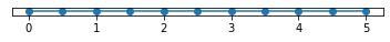
We can visually check the mesh using the FEniCS plot() command. The plot object is then displayed by adding the pyplot command show().

[173]:

fe.plot(mesh)
plt.show() # this forces the plot to show in a pop-up window when in command line/script environment

../_images/HeatEquation1D_wire1d_13_0.png

Weak formulation¶

As was said previously, any sensible nemerical simulation of a problem starts with its mathematical formulation, typically in the form of a PDE. This is sometimes called a classical formulation. Now more specifically, any finite element method computation starts with the so-called weak formulation of the problem, which stems from the PDE governing the problem, but should be understood rather as its generalization. One of the very nice features of FEniCS is that the implementation of the weak form closely imitates its (written) mathematical form. The weak formulation of our problem reads

\begin{align*} \text{look for } T \in V: a(T,\vartheta) = \mathscr{l}(\vartheta), \quad \forall \vartheta \in V\,, \end{align*}

where \(T(x)\) represents our weak solution, that is, the temperature field, \(\vartheta(x)\) is the so-called test function,

\begin{align*} a(T,\vartheta) = \int_0^L T'(x) \vartheta'(x)\, \text{d} x \end{align*}

is the bilinear form, that is a mapping \(a: V \times V \rightarrow \mathbb{R}\) linear in both of its arguments, and

\begin{align*} \mathscr{l}(\vartheta) = \int_0^L \frac{A^2 U^2}{\rho k} \vartheta(x)\, \text{d} x \end{align*}

is the linear functional defined on \(V\), which represents some linear space containing all the possible (weak) solutions to our problem1. Since the space \(V\) might be infinite dimensional, a crucial step of any numerical method, which begins with such formulation, is to approximate \(V\) using some smaller, i.e., finite-dimensional, space \(V_h\). The hallmark of FEM is that it uses piece-wise polynomial functions for the definition of \(V_h\).

Function spaces definition¶

Thus the first step in our FEniCS implementation of the finite element formulation is to define the proper function space approximation \(V_h\) that contains the piece-wise polynomial solution and test functions. This is done by initializing the object FunctionSpace(mesh,type,deg) with three arguments.

The first argument is the discretized domain contained in the mesh variable. Second and third are the type type of the base functions and the order deg of these functions respectively. We will present various types of function elements throughout this course. You can check an encyclopaedia of finite elements e.g., here. In this simple setting, we define the conforming space of finite elements, i.e., \(V \subset V_h\), or more specifically the Lagrange/Continous Galerkin element (hence the acronym CG) of order one, in other words, piecewise linear functions.

1It is the result of functional analytic approach to the theory of PDEs that such object is the Sobolev space \(H^1_0 = \{ v \in H^1(0,L); v(0) = v(L) = 0\}\). Further it holds that \(H^1(0,L) \subset AC[0,L]\) (which denotes the space of absolutely continuous functions on \([0,L]\)) meaning that it makes sense to use point-wise of the functions.

[174]:

# ---------
# FE spaces
# ---------
V_h = fe.FunctionSpace(mesh, "CG", 1)

Then, we need to initialize the solution and test functions (specified by the definition of \(V_h\)) as TrialFunction and TestFunction objects, respectively.

[175]:

# Definition of trial (=solution) and test functions:
_T = fe.TrialFunction(V_h)
Theta = fe.TestFunction(V_h)

Boundary conditions¶

As this next step, we specify the geometric boundary of the domain through which we apply the Dirichlet boundary conditions. It is necessary to mark those entities of the mesh that constitute the boundaries \(\Gamma_{\text{D}}\) and \(\Gamma_{\text{N}}\). This can be done essentially in two ways.

[176]:

# ------------------------
# Boundary markings
# ------------------------
def left(x, on_boundary):
    return fe.near(x[0], 0.0) and on_boundary
# analogously, we could define the marking of the right boundary
def right(x, on_boundary):
    return fe.near(x[0], L) and on_boundary

In the previous, on_boundary flag is True for all points that lie on the boundary of the mesh and near(x,x0) checks whether x is close to x0 (by default, within the tolerance given by the global constant DOLFIN_EPS), which respectively gives the left and the right end of the beam.

When you compare two real numbers in python, always use certain tolerance. Value of the tolerance depends on the size of the numbers you compare. For unit sized numbers, DOLFIN_EPS = 3e-16 is sufficient.

Try it for yourselves. Print the outcomes e.g., of 0.1+0.1+0.1-0.3 and 100.1+100.1+100.1-300.3:

[177]:

print(0.1+0.1+0.1-0.3)
print(100.1+100.1+100.1-300.3)

5.551115123125783e-17
-5.684341886080802e-14

There is an equivalent way of marking the boundary. It employs the MeshFunction object that represents a numerically/Boolean valued function defined on the mesh. More precisely, the first argument in initialization can either be ‘int’, ‘size_t’, or ‘double’, which denotes the integers, unsigned integers and floats, respectively. The Boolean valued function is initialized with the ‘bool’ argument.

[178]:

boundary = fe.MeshFunction("size_t", mesh, mesh.topology().dim()-1,0)
for v in fe.facets(mesh):
    if fe.near(v.midpoint()[0], 0.0):
        boundary[v] = 1 # left boundary
    elif fe.near(v.midpoint()[0], L):
        boundary[v] = 2 # right boundary

The previous for loop iterates through facets of the mesh (vertices in our example) and assigns the value one to the left boundary and the value two to the right boundary of the bar.

note: it is preferable to set some default numerical value (e.g., zero) to all the other mesh facets, this can be done either by giving the last optional argument 0 in the initialization of the MeshFunction object or by calling boundary.set_all(0) before the for loop

Though from the perspective of physics there are many boundary conditions (depending on what type of problem we solve), mathematically speaking all of the standard boundary conditions fall into one of the three following categories.

1. Dirichlet boundary conditions¶

The first type of boundary conditions is the one that prescribes some value of the solution at the boundary. With heat transfer problems, this constitutes the case when the boundary is held at a constant temperature, e.g., by a large reservoir of water.

note: In the realm of variational, or weak formulations of PDEs, the Dirichlet boundary conditions are sometimes called essential, since they determine the definition of the solution function space.

In FEniCS, Dirichlet boundary conditions are implemented through the object DirichletBC initialized with three arguments: the function space, the prescribed value at the boundary, and the corresponding subdomain specified by the previously defined left function (or equivalently by the boundary variable and its numerical value at the desired facets).

[179]:

# --------------------
# Boundary conditions
# --------------------
bc_left = fe.DirichletBC(V_h, T_c, left) # prescribe cellar temperature to the left end of the wire
bc_right = fe.DirichletBC(V_h, T_h, right) # prescribe outdoor temperature to the right end of the wire

# Group boundary conditions into an array:
bcs = [bc_left, bc_right]

# Equivalently, using boundary variable:
#bc_left = fe.DirichletBC(V_h, T_c, boundary, 1)
#bc_right = fe.DirichletBC(V_h, T_h, boundary, 2)

2. Neumann boundary conditions¶

The second type of boundary conditions specifies the value of the solution’s normal derivative across the boundary. For our physical problem, this means that the heat flux over the boundary is given by prescribed rate \(g\), i.e.,

\begin{align*} \mathbf{q} \cdot \mathbf{n} = -k \frac{\partial T}{\partial n} = g\,, \end{align*}

where \(\mathbf{n}\) denotes the outer unit normal (in our case \(-1\) for the boundary \(x = 0\) and \(+1\) for \(x = L\)), and \(g>0\) some given heat inflow through boundary.

note: The category of Neumann boundary conditions is sometimes denoted as natural. The natural boundary conditions are reflected directly in the weak formulation of the problem.

In the weak formulation above, the Neumann boundary condition would appear as a term from the integration by parts formula. To include this term in our implementation of the problem, we would first need to define the integrating measures that correspond to the boundary manifold of the mesh. To this end, we could initialize the Measure object with input arguments: string that specifies the integral type, "dx" for volume, "ds" for surface integral, and the respective geometry to which the measure corresponds, mesh for volume, boundary for surface integral.

[180]:

dx = fe.Measure("dx", mesh)
ds = fe.Measure("ds", subdomain_data = boundary)

3. Newton-Robin boundary conditions¶

The last class of boundary conditions represents a linear combination of the two previous kinds. Therefore both the solution’s value and its normal derivative are prescribed, mathematically

\begin{align*} aT + b \frac{\partial T}{\partial n} = g\,, \end{align*}

where \(a, b \in \mathbb{R}\) are arbitrary constants (weights). As the name might suggest, the convective heat transfer (Netwon’s law of cooling) can be described by this type of boundary condition. Namely

\begin{align*} \mathbf{q} \cdot \mathbf{n} = -k \frac{\partial T}{\partial n} = r\,(T_\infty - T)\,, \end{align*}

where \(r\) denotes the coefficient of heat transfer and \(T_\infty\) is the ambient temperature.

Discretized weak formulation and problem form¶

We are now ready to give the weak form of the problem. One of the very nice features of FEniCS is that the implementation closely imitates the weak formulation given above. Weak formulation is

\begin{align*} T - T_\mathrm{b} \in V_h: \sum_{i=1}^n\int_{x_{i-1}}^{x_i} T'(x) \vartheta'(x)\, \text{d} x = \sum_{i=1}^n\int_{x_{i-1}}^{x_i} \frac{A^2 U^2}{\rho k} \vartheta(x)\, \text{d} x, \quad \forall \vartheta \in V_h\,, \end{align*}

where \(V_h = \{ v \in C([0,L]); v(0) = v(L) = 0, v|_{[x_{i-1}, x_i]} \in P^1\}\), and \(T_\mathrm{b}\) is some particular solution that respects the boundary conditions, e.g., linear temperature distribution.

[181]:

# --------------------
# Weak form
# --------------------
#a = E*A*fe.inner(fe.grad(T),fe.grad(Theta))*dx
# One can equivalently write the bilinear form in this one-dimensional problem as
a = _T.dx(0)*Theta.dx(0)*fe.dx
l = A**2*U**2/(rho*k)*Theta*dx

We need to supply the subdomain measure ds with the value of the MeshFunction object that corresponds to the Neumann part of the boundary \(\Gamma_{\text{N}}\), i.e., two.

note: it is possible to access individual elements of the gradient grad of a function u via u.dx(i), where i specifies the derivative with respect to the i-th coordinate and the enumeration starts with zero, do not confuse this with the measure object dx that specifies the integration domain

dot(u,v) vs inner(u,v): FEniCS makes distinction between the inner product and dot product of two elements u, v, dot(u,v) contracts (sums) over the last index of the first element and the first index of the second element, whereas inner(u,v) sums over all indices of the elements that must be of the same order

if u, v are both vectors (rank 1 tensor), then dot(u,v)=inner(u,v)
matrix-vector multiplication \(\sigma \mathbf{n}\) is computed using dot(sigma,n)

Finally, we call the solver to compute the linear algebraic system generated by the finite element method. FEniCS is prompted to do that by calling the solve() function supplied with three parameters: linear variational equation, function that will store the resulting approximation and the problem specific Dirichlet boundary conditions.

Let us first introduce the function u that will contain the finite element solution. In the code environment we define the object Function pertaining to the function space \(V_h\). Then we can call solve(a==l, u, bc).

[182]:

# --------------------
# Solver
# --------------------
T = fe.Function(V_h)
fe.solve(a == l, T, bcs)
# Equivalent implementation:
# F = a-l
# problem = fe.LinearVariationalProblem(fe.lhs(F),fe.rhs(F),u,bc)
# solver = fe.LinearVariationalSolver(problem)

Post processing¶

There is more than one way of visualizing results from FEniCS computations, the readily available one is the tools offered by matplotlib library

Graphing with `matplotlib`¶

In the final stage of our simulation we visualize the computational results. This task is easily handled by the matplotlib library that we imported at the beginning and already used for mesh visualization.

[183]:

# --------------
# Postprocessing
# --------------

# Define exact solution:
x_ex = np.linspace(0, L, nx)
T_ex = [-(U*A)**2/(2*rho*k)*x_ex_i**2 + ((T_h-T_c)/L + (U*A)**2/(2*rho*k)*L)*x_ex_i + T_c for x_ex_i in x_ex]

# Graph solutions:
fe.plot(T-273.15)
plt.plot(x_ex, T_ex-273.15*np.ones(len(T_ex)), "x")
plt.xlabel("x [m]")
plt.ylabel("T [°C]")
plt.legend(["FEM solution","exact solution"])
plt.show()

../_images/HeatEquation1D_wire1d_34_0.png

Benchmarking results¶

For many trivial problems, ours included, there is an exact solution. We can use this solution to benchmark our numerical results. The previous cell introduced the visual comparison of the explicit and discretized solutions. To make the benchmarking process quantitative, we use FEniCS’ errornorm functionality. In order to benchmark the explicit solution, we first need to represent as an object that FEniCS can handle. Basically, there are two objects in the fenics library that are expedient to our goal.

Expression vs. UFL. FEniCS object Expression can be understood as an entity containing precise representation of some mathematical formula (e.g., the function \(\sin(x)\)), whereas UFL obejct is essentialy representation of that said formula that belongs to the finite element space \(V_h\). It is worth noting that anytime you want to work with expressions within the framework of FEM, you need to modify them so that they, again, belong to \(V_h\). This can also be done in two ways.

project vs interpolate. The result of interpolate is, simply put, a FE element function from V_h, that coincides with the original object in the nodes of the finite element (in our case of piece-wise linear functions, these are endpoints of every subinterval). projection on the other hand does not have to coincide in the nodal points, but it is in some sense the best approximation to the original object that lies in \(V_h\). More precisely it the result of the orthogonal projection of the object onto \(V_h\), mathematically it is a function u_h :nbsphinx-math:`in `V_h that satisfies

\begin{align*} \int_\Omega (u_h - \sin(x))v_h\,\mathrm{d}x = 0\,, \forall v_h \in V_h\,. \end{align*}

[184]:

# Define expression containg the explicit solution:
T_sol = fe.Expression("-U*U*A*A/(2.0*rho*k)*x[0]*x[0] + ((T_h - T_c)/L + U*U*A*A/(2*rho*k)*L)*x[0] + T_c",
                      U = U, A = A, rho = rho, k = k, T_h = T_h, T_c = T_c, L = L,
                     degree = 3)

#T_sol_prj = fe.project(T_sol, V_h)

# It is recommended to use a finer mesh for comparison:
mesh_fine = fe.IntervalMesh(3*nx, 0.0, L)

err = fe.errornorm(T_sol, T, mesh = mesh_fine)

print(err)

2.5805735030741737

Questions and excercises¶

Q.1 Are all the properties and variables really constant over the cross-section? Is the one-dimensional simplication justified? Q.2 Consider the wire to be thermally insulated on both ends, i.e., \(\partial T/\partial x(0) = \partial T/\partial x(L) = 0\), is such problem well defined? If not, how can we make it so?

E.1 Study the role of finite element degree, possibly on some coarse mesh. What should the graph of the solution look like? Based on the values of the error is it more efficient to raise degree of the finite element, or the number of the mesh nodes? E.2 Assume that the control unit (and effectively the left end of the wire) is cooled by a fan blowing air at the temperature \(T_0\), formulate the problem with this boundary condition. E.3 Try to the implement and test the formulation from Q.2. E.4 Study the difference between projection and interpolation on the step function

\[\begin{split}f(x) = \begin{cases} 0 & x <0 \\ 1/2 & x= 0 \\ 1 & x >0\end{cases}\end{split}\]

Complete code¶

[ ]:

# Import relevant modules:
import fenics as fe # 'import dolfin' does the same
import matplotlib.pyplot as plt
import numpy as np

# --------------------
# Parameters
# --------------------
# Geometric parameters:
L = 5.0  # Length of the wire [m]
R = 0.005 # Radius of the wire [m]
A = np.pi*R**2 # Cross-section area [m^2]

# Environment parameters:
T_c = 283 # Ambient temperature of the cellar [K]
T_h = 298 # Ambient temperature of the outside air [K]
U = 230 # Voltage drop [V]

# Material parameters:
rho = 1.68e-8 # Electrical resistivity of copper [Ω m]
k = 384.1 # Thermal conductivity of copper [W m^-1 K^-1]

# --------------------
# Geometry
# --------------------
nx = 10 # Number of mesh subintervals
mesh = fe.IntervalMesh(nx, 0.0, L)

fe.plot(mesh)
plt.show() # this forces the plot to show in a pop-up window when in command line/script environment

# ---------
# FE spaces
# ---------
V_h = fe.FunctionSpace(mesh, "CG", 1)

# Definition of trial (=solution) and test functions:
_T = fe.TrialFunction(V_h)
Theta = fe.TestFunction(V_h)

# ------------------------
# Boundary markings
# ------------------------
def left(x, on_boundary):
    return fe.near(x[0], 0.0) and on_boundary
# analogously, we could define the marking of the right boundary
def right(x, on_boundary):
    return fe.near(x[0], L) and on_boundary

boundary = fe.MeshFunction("size_t", mesh, mesh.topology().dim()-1,0)
for v in fe.facets(mesh):
    if fe.near(v.midpoint()[0], 0.0):
        boundary[v] = 1 # left boundary
    elif fe.near(v.midpoint()[0], L):
        boundary[v] = 2 # right boundary

# --------------------
# Boundary conditions
# --------------------
bc_left = fe.DirichletBC(V_h, T_c, left) # prescribe cellar temperature to the left end of the wire
bc_right = fe.DirichletBC(V_h, T_h, right) # prescribe outdoor temperature to the right end of the wire

# Group boundary conditions into an array:
bcs = [bc_left, bc_right]

# Define volume and surface measures:
dx = fe.Measure("dx", mesh)
ds = fe.Measure("ds", subdomain_data = boundary)

# --------------------
# Weak form
# --------------------
#a = E*A*fe.inner(fe.grad(T),fe.grad(Theta))*dx
# One can equivalently write the bilinear form in this one-dimensional problem as
a = _T.dx(0)*Theta.dx(0)*fe.dx
l = A**2*U**2/(rho*k)*Theta*dx

# --------------------
# Solver
# --------------------
T = fe.Function(V_h)
fe.solve(a == l, T, bcs)
# Equivalent implementation:
# F = a-l
# problem = fe.LinearVariationalProblem(fe.lhs(F),fe.rhs(F),u,bc)
# solver = fe.LinearVariationalSolver(problem)

# --------------
# Postprocessing
# --------------

# Define exact solution:
x_ex = np.linspace(0, L, nx)
T_ex = [-(U*A)**2/(2*rho*k)*x_ex_i**2 + ((T_h-T_c)/L + (U*A)**2/(2*rho*k)*L)*x_ex_i + T_c for x_ex_i in x_ex]

# Graph solutions:
fe.plot(T-273.15)
plt.plot(x_ex, T_ex-273.15*np.ones(len(T_ex)), "x")
plt.xlabel("x [m]")
plt.ylabel("T [°C]")
plt.legend(["FEM solution","exact solution"])
plt.show()

# Define expression containg the explicit solution:
T_sol = fe.Expression("-U*U*A*A/(2.0*rho*k)*x[0]*x[0] + ((T_h - T_c)/L + U*U*A*A/(2*rho*k)*L)*x[0] + T_c",
                      U = U, A = A, rho = rho, k = k, T_h = T_h, T_c = T_c, L = L,
                     degree = 3)

#T_sol_prj = fe.project(T_sol, V_h)

# It is recommended to use a finer mesh for comparison:
mesh_fine = fe.IntervalMesh(3*nx, 0.0, L)

err = fe.errornorm(T_sol, T, mesh = mesh_fine)

print(err)

Copper wire heating - ‘Hello World!’ example¶

Physical formulation¶

FEniCS Implementation¶

Problem parameters¶

Geometry of the problem¶

Weak formulation¶

Function spaces definition¶

Boundary conditions¶

1. Dirichlet boundary conditions¶

2. Neumann boundary conditions¶

3. Newton-Robin boundary conditions¶

Discretized weak formulation and problem form¶

Post processing¶

Graphing with `matplotlib`¶

Benchmarking results¶

Questions and excercises¶

Complete code¶

FEniCS fluid tutorial

Navigation

Related Topics

Copper wire heating - ‘Hello World!’ example¶

Physical formulation¶

FEniCS Implementation¶

Problem parameters¶

Geometry of the problem¶

Weak formulation¶

Function spaces definition¶

Boundary conditions¶

1. Dirichlet boundary conditions¶

2. Neumann boundary conditions¶

3. Newton-Robin boundary conditions¶

Discretized weak formulation and problem form¶

Post processing¶

Graphing with matplotlib¶

Benchmarking results¶

Questions and excercises¶

Complete code¶

Graphing with `matplotlib`¶