Navier Stokes - blood flow simulation
Formulation
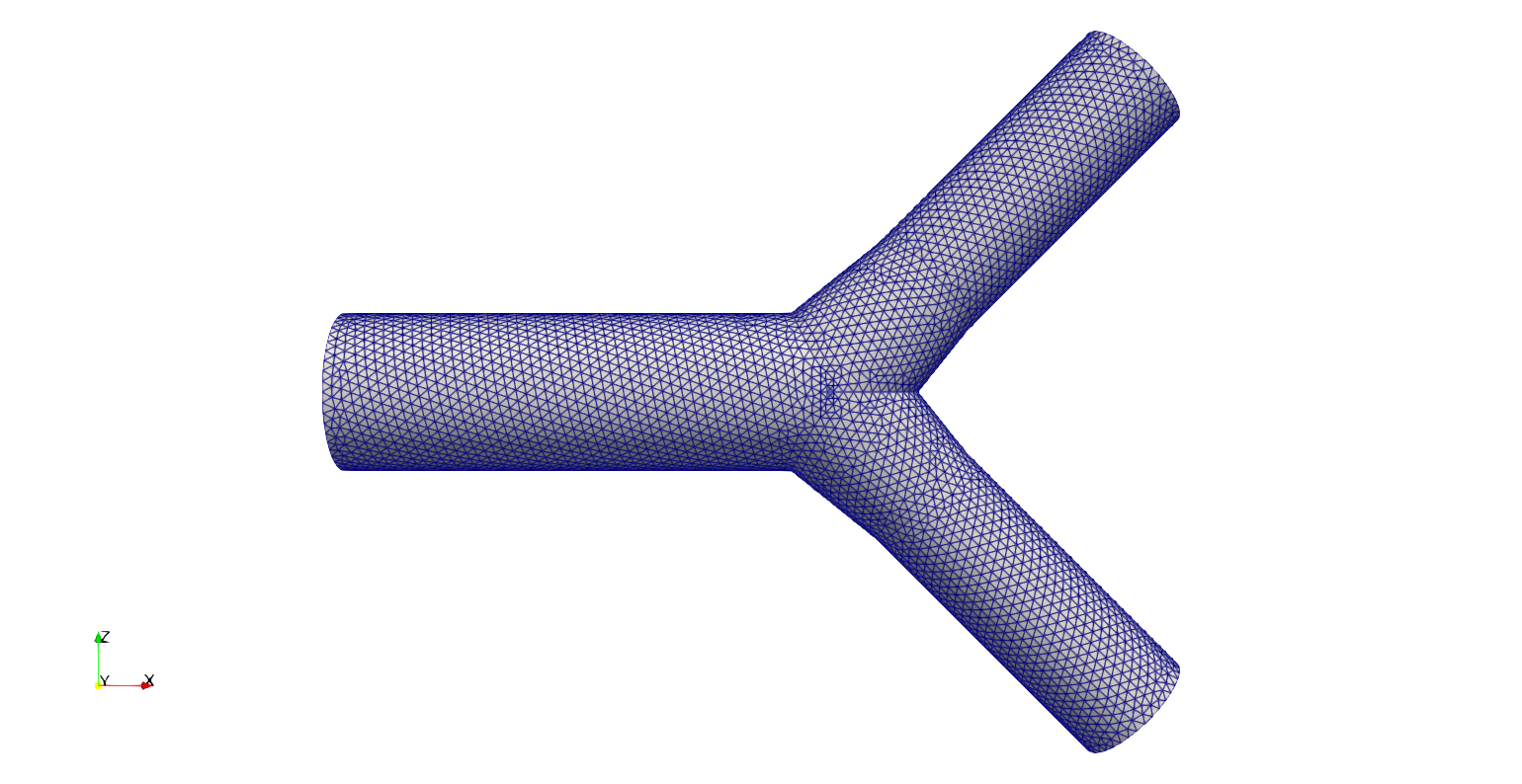
In this example we present a bloodflow simulation in a 3D geometry. The setting is very similar to the previous example. However, we will demonstrate how to prescribe a time dependent expression as a Dirichlet boundary condition. The inlet velocity is prescribed as
where \(r\) is the distance of the given point from the center point of the inlet. The average velocity at the inlet is changing over time according to the following equation
Implementation
Again, we need to import the neccessary packages.
[1]:
import dolfin as df
import numpy as np
from time import time
Next, we read the mesh from the file and create the boundary markings since .xml files do not include them. To do that, we create a mesh function and then loop over all the mesh facets and mark them in case they are a part of the desired boundary. We can save the marked mesh and open in ParaView.
[2]:
mesh = df.Mesh("bifurcation.xml")
dim = mesh.topology().dim()
bndry = df.MeshFunction("size_t", mesh, dim-1, 0)
mesh.init()

points = [np.array([-0.9, 0.0, 0.0]), np.array([0.6, 0.0, 0.6]), np.array([0.6, 0.0, -0.6])]
normals = [np.array([-1.0, 0.0, 0.0]), np.array([np.sqrt(2), 0.0, np.sqrt(2)]), np.array([np.sqrt(2), 0.0, -np.sqrt(2)])]
for f in df.facets(mesh):
    bndry[f] = 0
    if f.exterior():
        bndry[f] = 1
        x = f.midpoint().array() #[:dim]
        for mark, point, normal in zip([2,3,4], points, normals):
            if abs(np.dot(x-point, normal)) <= 0.001:
                bndry[f] = mark

with df.XDMFFile("marked_mesh.xdmf") as xdmf:
    xdmf.write(bndry)
Now we define the function spaces for MINI element as done in the previous example.
[3]:
U = df.FiniteElement("CG", mesh.ufl_cell(), 1)
B = df.FiniteElement("Bubble", mesh.ufl_cell(), dim + 1)
P = df.FiniteElement("CG", mesh.ufl_cell(), 1)
V = df.VectorElement(df.NodalEnrichedElement(U, B))
W = df.FunctionSpace(mesh, df.MixedElement([V, P]))
Let us define some parameters and constants such as density, dynamic viscosity, timestep size and time \(T\). The density and dynamic viscosity of blood are approximately \(\rho=1.05\,\frac{\text{g}}{\text{cm}^3}\) and \(\mu = 0.04\,\text{P (Poise)} = 0.004\,\text{Pa⋅s}\).
[4]:
mu = df.Constant(0.04) # Poise
rho = df.Constant(1.05) # g/cm^3
dt = 0.01
t_end = 0.35
Then we can define the boundary conditions as no slip on the wall and an expression at the inlet. Notice that the average inflow velocity is now prescribed using a function of time.
[5]:
zero_vector = df.Constant((0.0, 0.0, 0.0))
bc_walls = df.DirichletBC(W.sub(0), zero_vector, bndry, 1)

velocity = lambda t: 0.6*max((t*(0.3-t))/pow(0.15,2), 0.0)
inlet_expression = df.Expression(("v * 2.0 * (pow(R,2) - pow(x[0]-sx,2) - pow(x[1],2) - pow(x[2],2)) / pow(R,2)", "0.0", "0.0"), R=0.15, sx=points[0][0], v=velocity(0.0), degree=2)
bc_in = df.DirichletBC(W.sub(0), inlet_expression, bndry, 2)

bcs = [bc_in, bc_walls]
Then we can define the variational problem the same way as in the previous example.
[6]:
v, q = df.TestFunctions(W)
w = df.Function(W)
w0 = df.Function(W)
u, p = df.split(w)
u0, p0 = df.split(w0)

a = lambda u, v: rho*df.inner(df.grad(u)*u, v)*df.dx + mu*df.inner(df.grad(u), df.grad(v))*df.dx
b = lambda q, v: q*df.div(v)*df.dx

F1 = a(u, v) - b(p, v) - b(q, u)
F0 = a(u0, v) - b(p, v) - b(q, u)

theta = df.Constant(1.0) # Backward Euler
F = df.Constant(1.0/dt)*rho*df.inner((u-u0), v)*df.dx + theta*F1 + (1-theta)*F0
J = df.derivative(F,w)
We set up the nonlinear variational problem and solver.
[7]:
problem = df.NonlinearVariationalProblem(F, w, bcs, J)
solver = df.NonlinearVariationalSolver(problem)
solver.parameters['newton_solver']['linear_solver'] = 'mumps'
solver.parameters['newton_solver']['absolute_tolerance'] = 1e-8
solver.parameters['newton_solver']['relative_tolerance'] = 1e-6
Setup XDMF files to save results for viewing in Paraview.
[8]:
ufile = df.XDMFFile("results/u.xdmf")
pfile = df.XDMFFile("results/p.xdmf")
ufile.parameters["flush_output"] = True
pfile.parameters["flush_output"] = True
Again, we go over all the timesteps and solve for velocity and pressure at each of them using the solution from the previous timestep.
[ ]:
tick = time()
t = 0.0
(u, p) = w.split(True)
u.rename("v", "velocity")
p.rename("p", "pressure")
df.assign(u, w.sub(0))
df.assign(p, w.sub(1))
ufile.write(u, t)
pfile.write(p, t)
while t < t_end:
    w0.assign(w)
    t += dt
    print("t={:.2f}s".format(t))
    inlet_expression.v = velocity(t)
    solver.solve()
    df.assign(u, w.sub(0))
    df.assign(p, w.sub(1))
    ufile.write(u, t)
    pfile.write(p, t)
print("ellapsed = ", time() - tick, "s")
Complete Code
Run the code using the command python3 NavierStokes3D.py.
[ ]:
import dolfin as df
import numpy as np
from time import time

mesh = df.Mesh("bifurcation.xml")
dim = mesh.topology().dim()
bndry = df.MeshFunction("size_t", mesh, dim-1, 0)
mesh.init()

points = [np.array([-0.9, 0.0, 0.0]), np.array([0.6, 0.0, 0.6]), np.array([0.6, 0.0, -0.6])]
normals = [np.array([-1.0, 0.0, 0.0]), np.array([np.sqrt(2), 0.0, np.sqrt(2)]), np.array([np.sqrt(2), 0.0, -np.sqrt(2)])]
for f in df.facets(mesh):
    bndry[f] = 0
    if f.exterior():
        bndry[f] = 1
        x = f.midpoint().array()
        for mark, point, normal in zip([2,3,4], points, normals):
            if abs(np.dot(x-point, normal)) <= 0.001:
                bndry[f] = mark

with df.XDMFFile("marked_mesh.xdmf") as xdmf:
    xdmf.write(bndry)

U = df.FiniteElement("CG", mesh.ufl_cell(), 1)
B = df.FiniteElement("Bubble", mesh.ufl_cell(), dim + 1)
P = df.FiniteElement("CG", mesh.ufl_cell(), 1)
V = df.VectorElement(df.NodalEnrichedElement(U, B))
W = df.FunctionSpace(mesh, df.MixedElement([V, P]))

mu = df.Constant(0.04) # Poise
rho = df.Constant(1.05) # g/cm^3
dt = 0.01
t_end = 0.3

zero_vector = df.Constant((0.0, 0.0, 0.0))
bc_walls = df.DirichletBC(W.sub(0), zero_vector, bndry, 1)

velocity = lambda t: 0.6*max((t*(0.3-t))/pow(0.15,2), 0.0)
inlet_expression = df.Expression(("v * 2.0 * (pow(R,2) - pow(x[0]-sx,2) - pow(x[1],2) - pow(x[2],2)) / pow(R,2)", "0.0", "0.0"), R=0.15, sx=points[0][0], v=velocity(0.0), degree=2)
bc_in = df.DirichletBC(W.sub(0), inlet_expression, bndry, 2)

bcs = [bc_in, bc_walls]

v, q = df.TestFunctions(W)
w = df.Function(W)
w0 = df.Function(W)
u, p = df.split(w)
u0, p0 = df.split(w0)

a = lambda u, v: rho*df.inner(df.grad(u)*u, v)*df.dx + mu*df.inner(df.grad(u), df.grad(v))*df.dx
b = lambda q, v: q*df.div(v)*df.dx

F1 = a(u, v) - b(p, v) - b(q, u)
F0 = a(u0, v) - b(p, v) - b(q, u)

theta = df.Constant(1.0) # Backward Euler
F = df.Constant(1.0/dt)*rho*df.inner((u-u0), v)*df.dx + theta*F1 + (1-theta)*F0
J = df.derivative(F,w)

problem = df.NonlinearVariationalProblem(F, w, bcs, J)
solver = df.NonlinearVariationalSolver(problem)
solver.parameters['newton_solver']['linear_solver'] = 'mumps'
solver.parameters['newton_solver']['absolute_tolerance'] = 1e-8
solver.parameters['newton_solver']['relative_tolerance'] = 1e-6

ufile = df.XDMFFile("results/u.xdmf")
pfile = df.XDMFFile("results/p.xdmf")
ufile.parameters["flush_output"] = True
pfile.parameters["flush_output"] = True

tick = time()
t = 0.0
(u, p) = w.split(True)
u.rename("v", "velocity")
p.rename("p", "pressure")
df.assign(u, w.sub(0))
df.assign(p, w.sub(1))
ufile.write(u, t)
pfile.write(p, t)
while t < t_end:
    w0.assign(w)
    t += dt
    print("t={:.2f}s".format(t))
    inlet_expression.v = velocity(t)
    solver.solve()
    df.assign(u, w.sub(0))
    df.assign(p, w.sub(1))
    ufile.write(u, t)
    pfile.write(p, t)
print("ellapsed = ", time() - tick, "s")